Robust observations

An important drawback of standard least-squares algorithm such as Levenberg-Marquardt is that they assume that all observations are correct. Various types of estimators have been successfully used to deal with the presence of outliers in the data. Examples are least median-of-squares, RANSAC and Hough transform estimators. These estimators involve a radical redesign of the measurement error model. We employ what is probably the simplest method of ``robustifying'' the standard Gaussian error model. 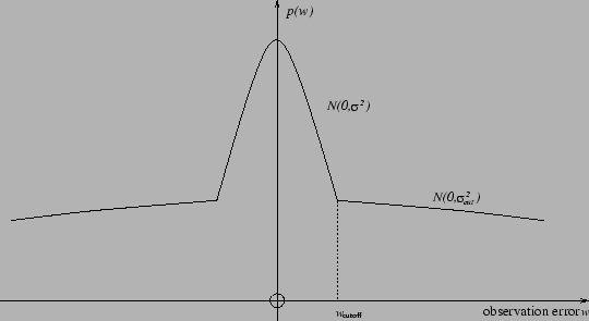The robust error model used here assumes that the errors follow a distribution combining a narrow ``inlier'' Gaussian with a wide ``outlier'' Gaussian, as shown for a one-dimensional distribution in Figure 5.4.

Figure 5.4: The error model used to model outliers in the observations incorporated in robust Levenberg-Marquardt, a combination of a narrow inlier Gaussian with variance $\sigma^2$, and wide Gaussian for outliers with variance $\sigma_{\rm out}^2$. Both distributions on the observation error $w$ have zero mean.

The distribution is a function of the observation error^5.3 ${\bf w}= {\bf z}- {\bf h}({\bf x})$. The relative vertical scaling of the two Gaussians is chosen so that the two distribution functions are equal at a chosen point $x_{\rm offset}$.

For a general multi-dimensional observation, we have a inverse covariance matrix $N^{-1}$ for the inlier distribution. We restrict the outlier distribution $N_{\rm out}^{-1}$ to be a rescaled version of the inlier distribution, so that

$$N_{\rm out}^{-1}= \frac{1}{V} N^{-1}$$

for some value $V>1$. We then set choose a cutoff hypersphere in the state space ${\bf x}$ for switching between the two distributions as a particular value of the $\chi^2$. So the probability distribution function is

$$p(\mbox{\boldmath$\nu$}) = \left\{ \begin{array}{ll} e^{-\mbo... ...dmath$\nu$}} & \mbox{otherwise (outlier)} \end{array} \right.$$

The scaling of the outlier distribution is chosen so that the two distributions are correctly aligned at the chosen cutoff point $\chi_{\rm cutoff}^2$. This leads directly to the correct ``compensation'' value for the likelihood function $1-K^{-1}\chi_{\rm cutoff}^2$, to be added to the least-squares residual when the outlier distribution is selected during application of a minimisation iteration. The simple scheme used to decide switching between the two distributions is detailed below. Note that each Levenberg-Marquardt observation can be chosen as robust or standard (non-robust), and potentially with a different choice for $K$ and $\chi_{\rm cutoff}^2$.